The cost of polynomial multiplication (including division) would quadratically depend on the input size if computed naively. Such dependence is not desirable for the efficiency of SNARKs and directly impacts proving performance.
For Parasol, this directly impacts throughput on Solana. At perpetual market scale, the gap between a quadratic and a near-linear algorithm compounds quickly.
In our previous article, we looked at a case where asymptotic improvements could be misleading - superlinear in theory, but could behave linear in practice. Here it's the opposite: the improvement is real, and it comes from using the structure of the problem in the right way.
The Fast Fourier Transform (FFT) addresses this by changing how polynomials are represented. In this article, we go through how this works and why it translates into a concrete speedup in practice.
The setup
Polynomial multiplication is a fundamental operation in computer science and mathematics, yet its straightforward implementation is surprisingly inefficient.
Given two polynomials of degree at most $n-1$, the naive method multiplies each coefficient of one polynomial with every coefficient of the other, leading to a quadratic running time of $\Theta(n^2)$. While acceptable for small inputs, this approach becomes prohibitively slow as $n$ grows.
The Fast Fourier Transform (FFT) provides a remarkable improvement, reducing the complexity of polynomial multiplication to $\Theta(n \log n)$ by reframing the problem in a different representation.
The method requires the field over which polynomials are defined to have at least 2n 2-primary roots of unity, i.e., solutions of $X^{2^r}=1$ for some positive integer $r$. Most fields don't satisfy this, which is one reason FRI-friendly fields like BabyBear and Mersenne31 are chosen the way they are (we covered this in our EdDSA series - part 1 and part 2). Note that Mersenne31 has only two 2-primary roots of unity but it has order one less than a high power of 2; hence it is known that FRI can be modified to operate there.
From coefficient to evaluations
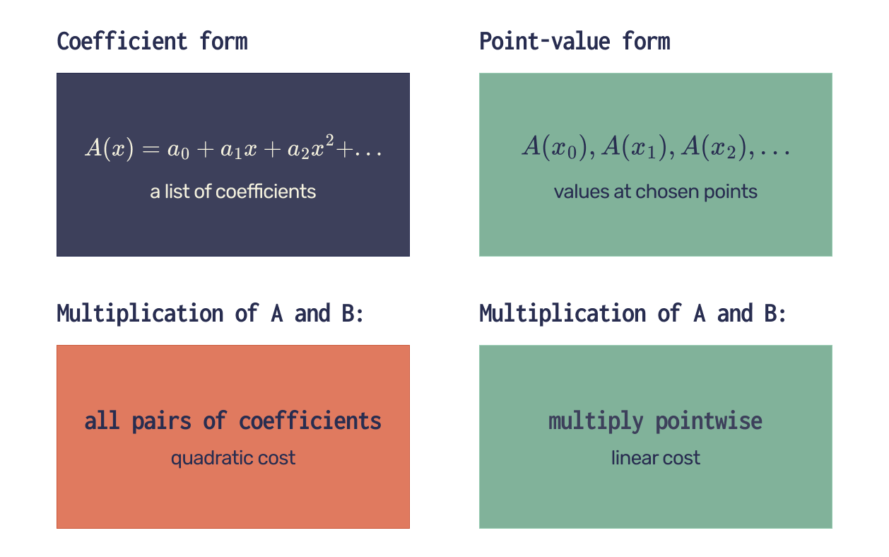
The key insight behind FFT-based multiplication is that polynomials can be expressed in two equivalent forms: the coefficient representation and the point-value representation. In the coefficient form, a polynomial is described by its coefficients, such as
$A(x) = a_0 + a_1x + \cdots + a_{n-1}x^{n-1}.$
This representation is natural and compact, but it makes multiplication expensive because it requires computing all pairwise products of coefficients. In contrast, the point-value representation describes a polynomial by its values at a set of distinct points. While this form is less intuitive, it has a crucial advantage: multiplying two polynomials $A$ and $B$ becomes trivial. If we know the values $A(x_k)$ and $B(x_k)$ at the same points $x_k$, then the product polynomial $C$ satisfies
$C(x_k) = A(x_k) \cdot B(x_k).$
Thus, multiplication reduces to pointwise multiplication, which takes only linear time.
Fast evaluation with FFT
The challenge, then, is to efficiently convert between these two representations. A naive approach to evaluating a polynomial at $n$ points or reconstructing it from those values takes $\Theta(n^2)$ time, which would negate any benefit. The FFT solves this issue by choosing a special set of evaluation points: $2$-primary roots of unity. These points possess rich algebraic structure and symmetry, which enable a divide-and-conquer algorithm for fast evaluation.
The FFT works by recursively decomposing a polynomial $A$ into two smaller polynomials $A^{[0]}$ and $A^{[1]}$ such that
$A(x) = A^{[0]}(x^2) + x \cdot A^{[1]}(x^2),$where $A^{[0]}$ and $A^{[1]}$ are polynomials of half the size. When evaluating at roots of unity, squaring these points effectively reduces the problem size by half. Each recursive step performs a linear amount of work, leading to the total work$T(n) = 2T(n/2) + \Theta(n) = \Theta(n \log n).$
Putting it together
Using the FFT, polynomial multiplication proceeds in four steps:
- Zero padding: the input polynomials are padded with zeros so that their degree bounds double, ensuring enough evaluation points for the product.
- Evaluation (FFT): both polynomials are evaluated at the chosen roots of unity using the FFT.
- Pointwise multiplication: their values are multiplied pointwise to produce the values of the product polynomial.
- Interpolation (inverse FFT): interpolate these values to obtain the coefficients of the product polynomial. The algorithm for the final step is called an inverse FFT, which itself is a particular instance of an FFT.
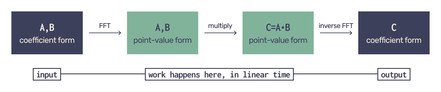
Both forward and inverse transforms run in $\Theta(n \log n)$ time, while the pointwise multiplication takes $\Theta(n)$, yielding an overall complexity of $\Theta(n \log n)$.
In essence, the FFT transforms polynomial multiplication into a problem that is easy in another domain and then efficiently converts the result back. This approach exemplifies a powerful algorithmic paradigm: change the representation, simplify the computation.
Beyond polynomial multiplication, the same ideas underpin fast convolution, signal processing, and many applications in engineering and data analysis. The FFT thus stands as one of the most important algorithms in computational mathematics, turning a seemingly intractable quadratic problem into a near-linear one.
This is the kind of structural insight that compounds at scale. Polynomial multiplication is one of many places in our proving pipeline where the right representation turns a quadratic cost into a near-linear one.
At the throughput that perpetual markets demand, those choices are what separate architecture that scales from one that becomes the bottleneck.